The voice app required the LLM to finish a response within a second while other calls were active. I started with a vanilla vLLM setup with light tuning, serving roughly 20 concurrent user streams as I recall. The optimized configuration handled 40 concurrent user streams at 500 ms model E2E p95 and 60 streams at around 800 ms on one B200.
I worked through CUDA graph coverage, speculative decoding, memory limits, and NVFP4 on Blackwell to support more concurrent user streams within the LLM latency budget.
The workload behind the one-second budget
I was serving a voice-agent workflow with several specialized agents, repeated prompt prefixes, and short responses. The one-second budget applied to a completed LLM request. Speech recognition, orchestration, and speech synthesis still took their own time before the caller heard a reply.
The workload used prompts of roughly 10,000 tokens, with responses of about 100 tokens.
Vanilla vLLM, lightly tuned
The starting point was a lightly tuned vanilla vLLM setup at roughly 20 concurrent user streams. That is my approximate recollection of the initial operating point, rather than a measured maximum. The optimized configuration later handled 40 concurrent user streams at 500 ms model E2E p95 and 60 streams at around 800 ms on one B200.
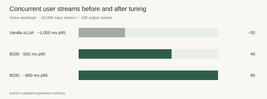
| Setup | Concurrent user streams | Model E2E p95 |
|---|---|---|
| Vanilla vLLM, lightly tuned | ~20 | ~1,000 ms |
| Optimized B200 · typical load | 40 | 500 ms |
| Optimized B200 · maximum tested load | 60 | ~800 ms |
The optimized setup handled 40 concurrent user streams at 500 ms model E2E p95 and 60 streams at around 800 ms on one B200, compared with the initial operating point of roughly 20 streams. These are complete serving configurations; the comparison does not assign a separate speedup to each optimization.
Capture the shapes the worker actually executes
A CUDA graph records GPU operations so the runtime can replay them with fewer CPU launch submissions. That helps when many small operations spend a meaningful fraction of their time waiting to be launched. The graph must cover the execution shape vLLM chooses for the batch.
I configured cudagraph_capture_sizes with dense coverage at small sizes and larger steps up to 16,384, using FULL_AND_PIECEWISE. The deployed recipe also used max_num_seqs=64, max_num_batched_tokens=16384, prefix caching, and chunked prefill. These limits describe different parts of scheduling; open user streams do not all occupy decoding slots at the same time.
# Extract from the recorded serving configuration
cudagraph_mode = "FULL_AND_PIECEWISE"
cudagraph_capture_sizes = (
    [1, 2, 4]
    + list(range(8, 257, 8))
    + list(range(272, 513, 16))
    + [640, 768, 1024, 1536, 2048, 3072,
       4096, 6144, 8192, 12288, 16384]
)
max_cudagraph_capture_size = 16384
Adding capture sizes gives vLLM more shapes to reuse, which can cut padding between them. It also adds startup time and memory. The useful range depends on the graph mode, attention backend, scheduled tokens, and speculative decoding. I would not copy a long-prompt capture list onto a decode-only workload without checking what gets replayed. The vLLM memory guide documents the memory tradeoff.
A startup OOM worth distinguishing from serving memory
The Hopper worklog documents a related failure on a hybrid Qwen model: the temporary KV allocation for graph profiling used the largest capture size as a count of cache blocks. Hybrid attention and recurrent-state storage shared a pool with unusually large blocks. A seemingly reasonable capture limit could therefore demand far too much temporary memory.
# The profiling allocation described in the Hopper investigation
min_blocks = self.compilation_config.max_cudagraph_capture_size or 1
self.cache_config.num_gpu_blocks_override = min_blocks
Their workaround capped the scratch allocation for their configuration. This is a version-specific debugging example, not a universal patch: the scratch cache must still cover the dummy forward pass. Before changing the main KV budget, inspect the allocation that actually fails.
Use MTP to get more useful tokens from a decoding step
Multi-token prediction, or MTP, supplies draft tokens that the target model verifies. When enough drafts are accepted, the worker advances by several tokens without repeating a full target-model step for each one. Drafting and verification also consume compute, so the useful setting depends on acceptance rate and load. vLLM exposes MTP through its speculative-decoding configuration.
--speculative-config '{"method":"mtp","num_speculative_tokens":4}'H200 and B200 change both capacity and bandwidth
At higher concurrency, memory has two separate jobs: hold the weights and live state, and deliver data quickly enough to keep decoding. More sequences increase state requirements. Longer contexts and larger graph pools compete for the same device memory. A workload can also miss its latency target while still having free memory, because transfers or computation cannot keep up.
H200 has 141 GB of HBM3e and 4.8 TB/s of bandwidth. NVIDIA lists 1,440 GB and 64 TB/s across eight GPUs for DGX B200, equivalent to 180 GB and 8 TB/s per GPU in that system. Those specifications explain the additional headroom; they do not predict an application speedup by themselves.
In my earlier FP8 sweep, H200 at 16 concurrent requests recorded p50 / p90 of 1.275 / 1.884 seconds. B200 at the same concurrency recorded 0.716 / 1.231 seconds. Both runs used FP8, so this predates any credit assigned to NVFP4. Hardware and backend selection can both contribute.
Use Blackwell's FP4 path
Blackwell adds native FP4 Tensor Core operations. FP4 represents a value with four bits; NVFP4 adds scales so small groups can represent different numerical ranges. It shares an FP8 scale across 16 values and uses another FP32 scale per tensor. Quantized values therefore take about 4.5 bits each before the tensor-scale overhead, rather than exactly four.
For tensors stored this way, that is roughly 1.8× less storage than FP8. Smaller weights reduce the data that must be moved, and compatible Blackwell kernels can execute low-precision matrix operations directly. The whole worker does not shrink by that factor: KV cache, recurrent state, activations, graph pools, and unquantized tensors still occupy memory.
My later B200 setup used Qwen3.5-35B-A3B NVFP4 quantization with modelopt_fp4, FP8 KV cache, and MTP4. In my newer tests at 40 concurrent user streams, the new quantization brought model E2E p95 from roughly 600 ms to 500 ms. That is about a 17% reduction in latency; the previous result was 20% higher than the new one.
What the complete setup handled
The starting point was about 20 concurrent streams at roughly 1,000 ms model E2E p95. The final setup reached 60 streams at around 800 ms: three times the concurrency, with a lower tail latency.
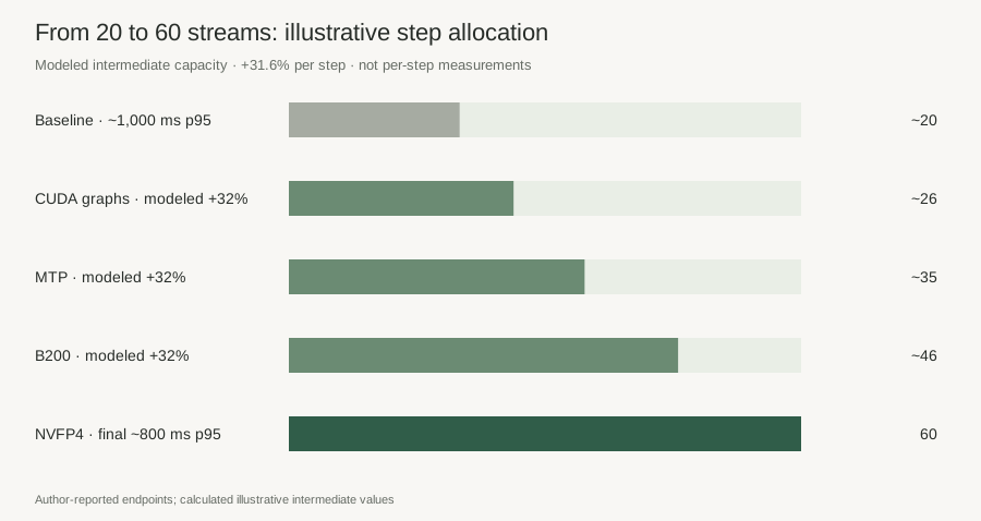
On one B200, the optimized configuration handled a typical load of 40 concurrent user streams at 500 ms model E2E p95. At the maximum tested load of 60 streams, p95 was around 800 ms, still within the one-second LLM budget.
E2E here measures a completed model request. Speech recognition, orchestration, and synthesis add their own latency before the user hears a reply.
Starting from roughly 20 user streams on lightly tuned vanilla vLLM, I worked toward a higher-load voice configuration. In the voice scenario, the NVFP4/MTP4 configuration handled 40 concurrent user streams at 500 ms model E2E p95 and 60 streams at around 800 ms on one B200. Graph coverage, speculative decoding, and the GPU/precision choice make up the serving recipe, but the saved runs do not break out an independent percentage for each step. That is the configuration and the load result I can carry forward.