In a voice call, the silence before the first word is part of the user experience. The speech model needs to start generating audio fast, keep the stream flowing without gaps, and do all of that while sharing the GPU with other active calls.
I built the serving stack around VITS, a compact speech model that fits well in voice pipelines and telephone workloads. I targeted single-GPU deployments on cards like the NVIDIA L4 and L40S. The main engineering task was turning the model into a streaming service that could serve many calls at once.
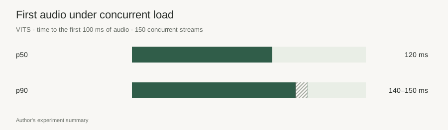
The optimized setup reached 150 concurrent streams with first-audio latency of 120 ms at p50 and 140–150 ms at p90, measured to the first 100 ms of audio. Getting there required changes to the model architecture, the computation graph, the precision, and the serving pipeline.
From a model invocation to a speech service
The initial setup ran the model through a PyTorch-based inference path. As I recall, it handled around 20 concurrent streams with responses on the order of a second. That was a workable baseline, but pushing concurrency higher made the behavior of the whole pipeline matter more.
I had three targets: cut the wait for the first audio chunk, keep subsequent chunks arriving fast enough for continuous playback, and support more simultaneous streams. Speeding up only the first response would not help if playback kept running out of audio.
The TTS team helped with model training and walked me through the architecture in detail. Their input helped me prepare for conversion and compilation. I then split the model and its surrounding processing into explicit modules, converted the neural parts for compiled inference, and assembled them into a service that could schedule work across active requests.
Give each stage its own execution path
The logical stages were text preprocessing, the encoder and acoustic path, the vocoder, and audio postprocessing. I made each one a separate serving component and connected them through a Triton ensemble.
With separate components, I could tune each part of synthesis independently. The encoder and vocoder used compiled engines, while preprocessing and postprocessing ran in backends suited to their specific work.
The preprocessing path also had a substantial neural component. I accelerated it with TensorRT-LLM and served it through its own backend as part of the ensemble. Since it sat on the path to the first sound, speeding up only the waveform generator would have left significant work untouched.
| Stage | Serving approach |
|---|---|
| Neural text preprocessing | TensorRT-LLM backend |
| Encoder / acoustic path | TensorRT engine |
| Vocoder | TensorRT engine |
| Audio postprocessing | Dedicated processing backend |
| Pipeline orchestration | Triton ensemble |
Compile the model and optimize its graph
I restructured the model architecture and computation graph during the TensorRT conversion. The converted neural components became compiled engines with explicit inputs and outputs, defining how stages connected in the pipeline.
The encoder and vocoder were natural boundaries for this. They run different computations on different tensor shapes. Splitting them into separate engines let me tune their execution independently and wire them together through a defined interface.
I also quantized model weights to FP8. That was one part of the optimization work, alongside the graph changes and compilation. I evaluated the serving configuration as a whole, so the final latency reflects the combined effect of those changes, not a percentage attributable to quantization alone.
TensorRT and TensorRT-LLM played distinct roles here. TensorRT handled the compiled speech-model components; TensorRT-LLM handled the neural preprocessing component. Triton connected those backends into the request path.
Batch work across streams, not whole conversations
The ensemble managed dependencies between stages. The backends handled their own execution and batching, combining compatible work from multiple requests. Requests moved through the pipeline asynchronously while work from other streams was in flight.
In a streaming service, requests don't arrive together or hit the same stage at the same time. One call might be in preprocessing while another is ready for the vocoder. A modular pipeline gives the scheduler more work to combine without treating an entire conversation as the execution unit.
Batching creates a tradeoff: waiting for a larger batch can improve GPU efficiency but delays the first chunk. I tuned the service around both startup latency and audio delivery during the stream, using concurrent calls as the workload.
First audio at 150 streams
At the highest load in these experiments, the system served 150 concurrent streams and delivered the first 100 ms of audio with a latency of 120 ms at p50 and 140–150 ms at p90. That is a service-level first-audio measurement, including the path through the ensemble.
The earlier operating point was roughly 20 streams with a response around a second. The result was reaching a much higher concurrent load while bringing the first audio forward. Those early figures are approximate, so I would not turn them into a precise latency-speedup ratio.
The distinction between initial delay and ongoing delivery stayed central. A caller can start listening after the first chunk arrives, but the pipeline then needs to keep the playback buffer supplied. That is why I worked on preprocessing, compiled model execution, batching, and postprocessing together.
Why this matters for a voice agent
A voice agent has several delay sources: recognizing the user, deciding what to say, generating text, synthesizing speech, and streaming the audio. Keeping TTS startup short gives the system more slack to respond naturally once the text is ready.
The VITS serving path became a practical fit for interactive LLM-driven calls. The compact model fit on a single GPU, and the ensemble let multiple active conversations share the same serving pipeline.
First-audio latency and real-time factor measure different things. RTF compares synthesis time against the duration of the generated audio. The first-audio percentiles and the stream count describe responsiveness under load; calculating RTF requires the full synthesis timing and the audio duration.
Finding the bottlenecks with NVIDIA Nsight
I used NVIDIA Nsight to track down the bottlenecks. A request-level timer showed how long a caller waited, and profiling showed what the CPU and GPU were doing inside that interval.
The Nsight Systems timeline links CPU-side CUDA calls to GPU kernel execution and memory transfers. That made it easier to separate computation from launch overhead, synchronization, and time spent waiting between stages.
I used the profiling results to guide the graph and serving work, then checked the full pipeline under concurrent load. The question was whether a change brought the first audio forward and kept the service producing the next chunks as more calls arrived.